To obtain the data to run this tutorial, download the tar.gz file from https://zenodo.org/records/10668525 and unzip it. Then set simulation_directory to point to the resulting directory.

Reading raw simulation files

Simulations do not have to be fully stitched into an h5 file before reading and visualzing their data

from mayawaves.utils.postprocessingutils import get_stitched_data
import matplotlib.pyplot as plt
import numpy as np

simulation_directory = "D11_q5_a1_-0.362_-0.0548_-0.64_a2_-0.0013_0.001_-0.0838_m533.33"

Use get_stitched_data to stitch together any output file structured as columns of data with each row being a time/iteration step

shifttracker0_data = get_stitched_data(simulation_directory, 'ShiftTracker0.asc')
shifttracker1_data = get_stitched_data(simulation_directory, 'ShiftTracker1.asc')

Stitching 17 files
Stitching 17 files

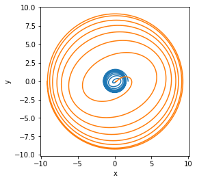
You can then plot the data based on the columns present in the data file. In the following, columns 2 and 3 (starting at 0) of the shift tracker files contain the x and y components of the positions.

plt.plot(shifttracker0_data[:,2], shifttracker0_data[:,3])
plt.plot(shifttracker1_data[:,2], shifttracker1_data[:,3])
plt.gca().set_aspect('equal', adjustable='box')
plt.xlabel('x')
plt.ylabel('y')
plt.show()

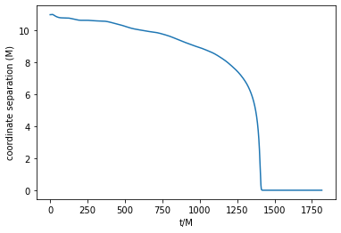
separation_vector = shifttracker1_data[:,2:5] - shifttracker0_data[:,2:5]
separation_mag = np.linalg.norm(separation_vector, axis=1)

plt.plot(shifttracker0_data[:,1], separation_mag)
plt.xlabel('t/M')
plt.ylabel('coordinate separation (M)')
plt.show()

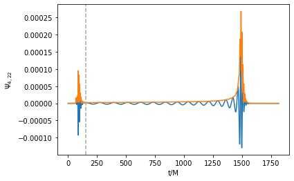
Plot the real componenet of the \(\Psi_4\) data using columns 0 and 1 of the Ylm_WEYLSCAL4 files

Note that the initial ~(75 + extraction_radius) M will be junk radiation and should be cut off for most analyses. That time is marked in the following tutorial with a vertical dashed line.

psi4_data = get_stitched_data(simulation_directory, 'Ylm_WEYLSCAL4::Psi4r_l2_m2_r75.00.asc')

Stitching 17 files

plt.plot(psi4_data[:,0], psi4_data[:,1])
plt.plot(psi4_data[:,0], np.sqrt(psi4_data[:,1]*psi4_data[:,1] + psi4_data[:,2]*psi4_data[:,2]))
plt.axvline(x=150, c='#a9a9a9', linestyle='--')
plt.xlabel('t/M')
plt.ylabel(r'$\Psi_{4, 22}$')
plt.show()