To obtain the data to run this tutorial, download the tar.gz file from https://zenodo.org/records/10668525 and unzip it. Then run the creating_h5 tutorial to create a .h5 file to use with this tutorial. Then set example_h5_filepath to be the path to that .h5 file.

Once you have run the tutorial on the sample simulation, you can also try downloading a file from the MAYA catalog in the MAYA format (https://cgp.ph.utexas.edu/waveform) and using it with the tutorial.

Compact Objects

from mayawaves.coalescence import Coalescence
from mayawaves.compactobject import CompactObject
import matplotlib.pyplot as plt

Create a Coalescence object using the simulation h5 file

example_h5_filepath = "D11_q5_a1_-0.362_-0.0548_-0.64_a2_-0.0013_0.001_-0.0838_m533.33.h5"

coalescence = Coalescence(example_h5_filepath)

Obtain the CompactObject objects associated with the larger object (primary) and smaller object (secondary)

primary_compact_object = coalescence.primary_compact_object
secondary_compact_object = coalescence.secondary_compact_object

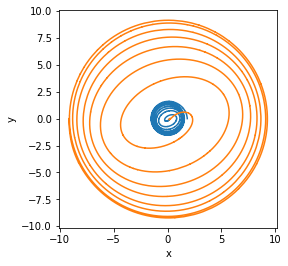
Obtain trajectory data

time, primary_position = primary_compact_object.position_vector
time, secondary_position = secondary_compact_object.position_vector

plt.plot(primary_position[:, 0], primary_position[:, 1])
plt.plot(secondary_position[:, 0], secondary_position[:, 1])
plt.gca().set_aspect('equal', adjustable='box')
plt.xlabel('x')
plt.ylabel('y')
plt.show()

Obtain initial data such as masses and spins

print(f"initial dimensionless spin of primary BH: {primary_compact_object.initial_dimensionless_spin}")
print(f"initial dimensionless spin of secondary BH: {secondary_compact_object.initial_dimensionless_spin}")
print(f"initial dimensional spin of primary BH: {primary_compact_object.initial_dimensional_spin}")
print(f"initial dimensional spin of secondary BH: {secondary_compact_object.initial_dimensional_spin}")

initial dimensionless spin of primary BH: [-0.36451101 -0.05518085 -0.64443774]
initial dimensionless spin of secondary BH: [-0.00129516  0.00100747 -0.08374188]
initial dimensional spin of primary BH: [-0.25138458 -0.0380554  -0.4444357 ]
initial dimensional spin of secondary BH: [-3.59770435e-05  2.79857020e-05 -2.32619237e-03]

print(f"initial horizon mass of primary BH: {primary_compact_object.initial_horizon_mass}")
print(f"initial horizon mass of secondary BH: {secondary_compact_object.initial_horizon_mass}")
print(f"initial irreducible mass of primary BH: {primary_compact_object.initial_irreducible_mass}")
print(f"initial irreducible mass of secondary BH: {secondary_compact_object.initial_irreducible_mass}")

initial horizon mass of primary BH: 0.8304509510300787
initial horizon mass of secondary BH: 0.16666770757317356
initial irreducible mass of primary BH: 0.7588330514
initial irreducible mass of secondary BH: 0.166521231

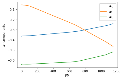
Obtain timeseries data for parameters such as spin

Note that for many systems, the initial horizons are tracked all the way through merger after which the values are no longer reliable.

time, primary_spin = primary_compact_object.dimensionless_spin_vector

plt.plot(time, primary_spin[:, 0], label=r'$a_{1, x}$')
plt.plot(time, primary_spin[:, 1], label=r'$a_{1, y}$')
plt.plot(time, primary_spin[:, 2], label=r'$a_{1, z}$')
plt.legend()
plt.xlabel('t/M')
plt.ylabel(f'$a_{1}$ components')
plt.show()

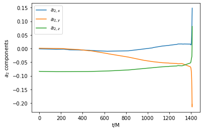
time, secondary_spin = secondary_compact_object.dimensionless_spin_vector

plt.plot(time, secondary_spin[:, 0], label=r'$a_{2, x}$')
plt.plot(time, secondary_spin[:, 1], label=r'$a_{2, y}$')
plt.plot(time, secondary_spin[:, 2], label=r'$a_{2, z}$')
plt.legend()
plt.xlabel('t/M')
plt.ylabel(f'$a_{2}$ components')
plt.show()

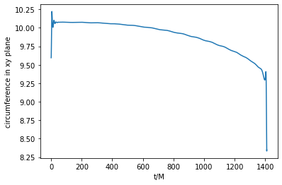
You can access any data that is available for the given compact object

available_columns = primary_compact_object.available_data_columns
print(available_columns)

[<Column.ITT: 1>, <Column.TIME: 2>, <Column.X: 3>, <Column.Y: 4>, <Column.Z: 5>, <Column.VX: 6>, <Column.VY: 7>, <Column.VZ: 8>, <Column.AX: 9>, <Column.AY: 10>, <Column.AZ: 11>, <Column.SX: 12>, <Column.SY: 13>, <Column.SZ: 14>, <Column.PX: 15>, <Column.PY: 16>, <Column.PZ: 17>, <Column.MIN_RADIUS: 18>, <Column.MAX_RADIUS: 19>, <Column.MEAN_RADIUS: 20>, <Column.QUADRUPOLE_XX: 21>, <Column.QUADRUPOLE_XY: 22>, <Column.QUADRUPOLE_XZ: 23>, <Column.QUADRUPOLE_YY: 24>, <Column.QUADRUPOLE_YZ: 25>, <Column.QUADRUPOLE_ZZ: 26>, <Column.MIN_X: 27>, <Column.MAX_X: 28>, <Column.MIN_Y: 29>, <Column.MAX_Y: 30>, <Column.MIN_Z: 31>, <Column.MAX_Z: 32>, <Column.XY_PLANE_CIRCUMFERENCE: 33>, <Column.XZ_PLANE_CIRCUMFERENCE: 34>, <Column.YZ_PLANE_CIRCUMFERENCE: 35>, <Column.RATIO_OF_XZ_XY_PLANE_CIRCUMFERENCES: 36>, <Column.RATIO_OF_YZ_XY_PLANE_CIRCUMFERENCES: 37>, <Column.AREA: 38>, <Column.M_IRREDUCIBLE: 39>, <Column.AREAL_RADIUS: 40>, <Column.EXPANSION_THETA_L: 41>, <Column.INNER_EXPANSION_THETA_N: 42>, <Column.PRODUCT_OF_THE_EXPANSIONS: 43>, <Column.MEAN_CURVATURE: 44>, <Column.GRADIENT_OF_THE_AREAL_RADIUS: 45>, <Column.GRADIENT_OF_THE_EXPANSION_THETA_L: 46>, <Column.GRADIENT_OF_THE_INNER_EXPANSION_THETA_N: 47>, <Column.GRADIENT_OF_THE_PRODUCT_OF_THE_EXPANSIONS: 48>, <Column.GRADIENT_OF_THE_MEAN_CURVATURE: 49>, <Column.MINIMUM_OF_THE_MEAN_CURVATURE: 50>, <Column.MAXIMUM_OF_THE_MEAN_CURVATURE: 51>, <Column.INTEGRAL_OF_THE_MEAN_CURVATURE: 52>]

data = primary_compact_object.get_data_from_columns([CompactObject.Column.TIME, CompactObject.Column.XY_PLANE_CIRCUMFERENCE])
time = data[:, 0]
circumference = data[:, 1]
plt.plot(time, circumference)
plt.xlabel('t/M')
plt.ylabel('circumference in xy plane')
plt.show()

Close the Coalescence object to close the associated h5 file

coalescence.close()